Deduplication Pipelines With Pandas and Recordlinkage

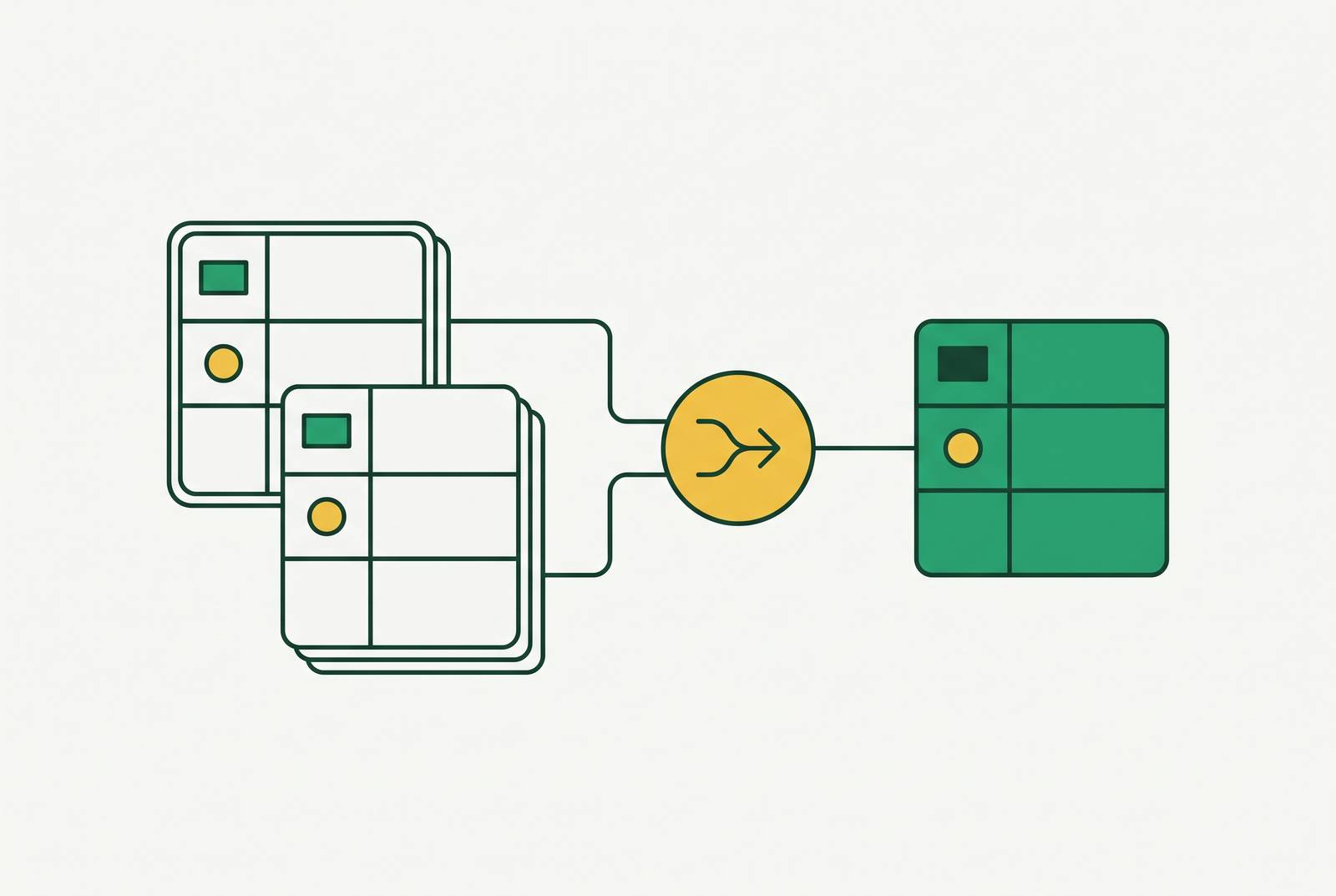
Deduplication pipelines with pandas and recordlinkage depend on clear handoffs between preparation, candidate generation, comparison, classification, and canonicalization. Pandas prepares the records and builds the final dataset, while recordlinkage identifies likely matches. Production reliability comes from treating those stages as one connected process, because an error introduced early can survive every later step.

Why duplicate records are harder to catch than they look

Exact duplicates and near-duplicates require different kinds of evidence. Exact duplicates match identically across every field, so removing them is a straightforward equality operation. Near-duplicates are records for the same real-world entity, but their spelling or formatting differs, or some attributes are missing. Equality alone cannot resolve that second group. Two rows can disagree without representing different people, just as a shared name does not establish that two contacts are identical.

These differences often originate in the source systems. Manual entry introduces spelling errors, while CRMs, APIs, event logs, and payment platforms can store the same entity in different forms. In a CRM or RevOps dataset, separate records for one contact distort engagement scoring and pipeline reporting. AI agents working from those records can then produce confident but wrong outputs.

Rebecca C. Steorts’s A Primer on the Data Cleaning Pipeline defines four stages, which are schema alignment, blocking, entity resolution, and canonicalization. The primer establishes that errors propagate from one stage into the next. Near-duplicate detection therefore requires more than a better deletion rule. It requires a multi-stage process, which the pandas and recordlinkage combination provides.

How pandas and recordlinkage divide the work between them

Pandas handles the tabular work that makes records comparable. It reads sources, aligns columns and types, and normalizes values into a consistently structured DataFrame. Recordlinkage then uses that DataFrame directly because it uses pandas and numpy internally. No intermediate format conversion is needed. The first handoff is therefore a data-quality boundary.

Within recordlinkage, an indexer generates candidate pairs, a comparator scores their fields, and a classifier decides which pairs are matches. Each object produces the input for the next. Pandas returns at the end to collapse matched clusters into canonical records.

This division also explains two common structural failures. When matching tools work on raw data, differences in formatting can rule out true matches before scoring begins. Trying to perform every pairwise comparison directly in pandas, without candidate generation, avoids neither the computational cost nor the need for explicit classification.

Stage one: loading and normalizing data with pandas

Ingestion begins with pd.read_csv(), pd.read_sql(), or the equivalent operation for the source. The required output is a DataFrame with one record per row and consistently typed attributes in its columns. Reading the data is only the start. String fields need deliberate casing and whitespace rules, dates need consistent formats, and nulls need to be filled or flagged. Sources that split first and last names must also align with sources that provide a full-name field.

Exact duplicates can be removed with drop_duplicates(), but the selection rule needs care. With keep='first', the retained row depends on input order, which can change between ingestions. For fully identical rows, that does not change their field values, but row selection still needs a reproducible basis for tracing what happened. A sort-before-dedup expression is df = df.sort_values(['user_id', 'event_id', 'timestamp']).drop_duplicates(keep='first'). The sorting key must establish the stable ordering that “first” is intended to mean.

Removed rows and the reason for removal should be logged, so duplicate ingestion can be traced to an ETL problem, source misconfiguration, or historical replay. Near-duplicates remain intact at this stage. Memory also constrains ingestion before matching begins. When the dataset will not fit in one DataFrame, SQL-native deduplication or chunked processing is needed before constructing the in-memory working dataset.

Stage two: generating candidate pairs with blocking

When every record is compared with every other record, the work grows at a quadratic rate. Blocking reduces that work by admitting only pairs that share a selected value. It is also a recall decision. A true duplicate excluded here never reaches the comparator, regardless of how good the later scoring model is.

For a single dataset, the basic sequence is indexer = recordlinkage.Index(), then indexer.block("given_name"), followed by candidate_pairs = indexer.index(df). The resulting candidate_pairs is a pandas MultiIndex. Each entry has two record index values that show which rows to compare. It contains no similarity scores and makes no match decision. The same indexer can generate cross-dataset pairs when linking two datasets.

The blocking key determines which disagreements the pipeline can tolerate. An unnormalized name can keep true matches apart, while email blocking misses duplicates when their email values differ. Multiple overlapping passes, such as one on first name and another on postcode, can improve recall by taking the union of their candidate pairs. That broader coverage costs additional comparisons.

The BlockingPy paper shows why deterministic blocking can fail: it assumes that blocking variables have no errors or missing values. BlockingPy uses approximate nearest neighbour search to find candidates through vector similarity, so fields do not have to match by exact field equality. It is a possible complement when dirty blocking fields produce unacceptable miss rates.

Stage three: comparing candidate pairs field by field

The comparator transforms each candidate pair into a feature vector, with a separate similarity value for each selected field. Those values are evidence. String comparisons such as Jaro-Winkler or Levenshtein express degrees of similarity between 0 and 1. Exact comparisons instead represent agreement or disagreement, which suits identifiers and categorical codes where partial similarity has no useful meaning.

A compact comparison sequence begins with compare = recordlinkage.Compare(). A name feature can be added with compare.string("given_name", "given_name", method="jarowinkler", label="given_name"), and a categorical feature with compare.exact("country_code", "country_code", label="country_code"). The call features = compare.compute(candidate_pairs, df) produces a DataFrame indexed by the candidate-pair MultiIndex. Each column now shows the comparison for one field. Additional relevant fields give the classifier more evidence than this minimal sketch.

Method selection must follow the meaning of the attribute. Jaro-Winkler weights prefix agreement, while numeric comparisons are useful where near-equality is a meaningful signal and date comparisons address date-specific differences. Digits in a field alone do not show that numerical proximity is useful evidence.

Normalization determines how much that evidence can be trusted. An exact city comparison between “new york” and “New York” scores 1.0 only after consistent lowercasing, rather than 0.0 on the unnormalized strings. Comparing too few attributes also weakens discrimination. The classifier cannot recover useful distinctions that the feature matrix never expresses.

Stage four: classifying pairs as matches or non-matches

Classification converts each feature vector into a match or non-match decision. The main choice is whether labeled examples are available. With manually verified pairs, recordlinkage.LogisticRegressionClassifier or recordlinkage.SVMClassifier can learn domain-specific distinctions. Supervised approaches typically outperform unsupervised ones on domain-specific data when suitable labels are available. The scikit-learn integration also permits an sklearn-compatible classifier to be used with training data.

Without training labels, ECM provides an unsupervised route. For a feature matrix prepared for that classifier, the call sequence is ecm = recordlinkage.ECMClassifier() followed by matched_pairs = ecm.fit_predict(features). ECM is closely related to estimating parameters in the Fellegi-Sunter probabilistic framework, which uses comparison evidence to distinguish matches from non-matches. The resulting matched_pairs is another MultiIndex, now containing pairs classified as matches.

The operating threshold depends on how much mistakes cost. A false positive merges separate entities, while a false negative leaves a duplicate unresolved. For CRM deduplication, incorrectly merging distinct contacts is typically more damaging, so higher precision is usually the appropriate preference. A small validation set labeled by hand can help calibrate the threshold before deployment. Recordlinkage provides precision, recall, and F1 evaluation tools against ground-truth pairs, making that tradeoff measurable.

Stage five: merging matched clusters back into pandas

Matched pairs form a graph in which records are nodes and predicted matches are edges. Connected components group those relationships into clusters for canonicalization. Python’s networkx or a union-find algorithm can perform that step. Because the edges are predictions, clustering does not remove the consequences of a classification error.

A sketch in networkx starts with graph = nx.Graph(), adds the records with graph.add_nodes_from(df.index), and adds the relationships with graph.add_edges_from(matched_pairs). The call components = nx.connected_components(graph) then identifies the groups. Including all record indexes preserves unmatched records as well. A mapping from source record index to cluster identifier gives pandas the information needed to combine the groups.

For a most-recent-record policy, a pandas sketch is tagged = df.merge(cluster_map, left_index=True, right_index=True), followed by canonical = tagged.sort_values("timestamp").drop_duplicates("cluster_id", keep="last"). That policy is not universally correct. Another business may keep the most complete row or combine non-null fields, using a source-of-truth hierarchy to choose between values that disagree. Each decision needs a rule for whether to trust the CRM system of record or the marketing tool, or to use completeness or recency.

The primer defines canonicalization as the stage that “attempts to repair any errors from previous stages to output a single integrated data set, with a unique identifier for each record”. Each canonical entity therefore needs a stable identifier. Keeping a log of the source IDs collapsed into that entity helps with audits and with tracing what went wrong when downstream results look wrong.

Where this pipeline breaks and what to do about it

Blocking reduces pair counts but does not guarantee manageable workloads. Within large blocks, comparison work can still grow at a quadratic rate, so the pipeline can hit timeouts or run out of memory. The candidate count is the early warning. Before comparison, the pipeline should validate that count and, where necessary, use tighter rules or multiple narrow passes. At very large scale, Splink with a DuckDB or Spark backend represents an architectural alternative to an in-memory pipeline.

Sorting addresses row-order instability, but it cannot protect against renamed columns, changed types, or altered null patterns. A schema check immediately after ingestion should validate expected column names, types, and null rates before normalization begins. Without that boundary, later stages can operate on inputs that no longer mean what their rules assume.

Classification needs its own ongoing checks because a threshold calibrated on earlier data can become unsuitable as sources, naming conventions, or geographies change. Regular checks against a held-out labeled set should raise an alert when precision or recall falls below a set floor. Threshold tuning is an operational responsibility. A successful initial evaluation does not establish that future similarity distributions will behave the same way.

Auditability connects these controls to downstream repair. To find out reliably why a merge was wrong, the pipeline needs a record of what changed and why. Missing lineage also obstructs right-to-erasure requests when deleting one record leaves duplicate copies of personal data behind. Production discipline therefore includes both reproducible decisions and a trace from canonical entities back to the source records involved.

Why a deduplication pipeline is not a one-time job

New records arrive after the first cleanup, and source systems continue producing duplicates. Contacts change roles, companies merge, and records that once were useful become stale. Clean output does not maintain itself. The pipeline must run on a schedule, with its results monitored as part of data reliability.

For AI and RevOps workflows, repeated records change the weight assigned to an entity. Duplicate examples receive disproportionate influence in model training, while duplicate contacts distort scoring and pipeline aggregations. Detecting those records only at consumption leaves the same underlying error available to other downstream systems. Embedding checks at ingestion shifts correction earlier, before duplicates spread into models, dashboards, and workflows.

The same architecture can keep that process running with normalization on a schedule, incremental blocking against new records, and automated flagging of records for review or resolution. Agentic approaches take on the same work by watching systems of record and suggesting or applying fixes as duplicates arrive. Their usefulness still depends on the stage boundaries described here, because autonomous execution cannot compensate for candidates never generated, weak comparison evidence, or an undefined source-of-truth policy.